What Is LLM Quantization?

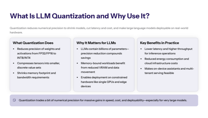
Quantization is the process of reducing the numerical precision used to represent a model’s parameters and intermediate values—from high-precision floating-point representation (e.g., FP32/FP16/BF16) to lower precision formats such as INT8, INT4, or even ternary/binary. For large language models (LLMs), this kind of model quantization can shrink memory footprint, improve throughput, and cut energy use, enabling deployment on resource-constrained hardware while keeping model accuracy within acceptable bounds.

In practice, quantization converts continuous real-valued model weights and activations into a small, fixed set of quantized data values. The quantization procedure can be applied after training (PTQ), during training (quantization-aware training, QAT), or at runtime (dynamic quantization) depending on your latency/quality trade-offs.

Because LLMs are deep neural networks with billions of parameters, the impact of precision reduction is multiplicative—smaller tensors mean less memory traffic and less computational costs, which often dominates inference time. The challenge is to achieve quantization with minimal accuracy loss; doing so reliably is the core of modern quantization methods research.

Why Quantize Large Language Models?

Quantization addresses three practical issues that arise when serving LLMs at scale:

1. Memory & bandwidth. Quantized weights require fewer bytes, reducing VRAM and memory bandwidth pressure. On many accelerators, memory movement—not compute—is the bottleneck.

2. Latency & throughput. Integer matrix multiplies can be faster than floating-point, and smaller activations speed up memory-bound kernels.

3. Cost & energy. Lower precision reduces power draw and cloud spend, while enabling smaller models on embedded devices.

These gains unlock use cases like on-device assistants and low-latency chat, where computational power is limited, and allow multi-tenant serving of very large checkpoints.

How Does Quantization Work? Affine Quantization

Most production systems use affine quantization. Real values x are mapped to integers q using a scaling factor s and a zero point z:

q = \text{round}\!\left(\frac{x}{s}\right) + z,\qquad \hat{x} = s\,(q - z)

Here, s expands a discrete integer range (e.g., [0,255] for INT8) into a continuous interval, and z aligns the integer zero with the real zero. Choosing s and z requires range estimation from data: you determine minimum and maximum values (or robust statistics) for a tensor and map them to the representable symmetric range (e.g., [-128,127]) or an asymmetric range (e.g., [0,255]).

This mapping is applied to weight quantization (persistent parameters) and activation quantization (layer outputs). The inevitable quantization error—the difference between x and \hat{x}—must be controlled to preserve model accuracy.

Floating-Point vs. Lower Precision Formats

• FP32 / FP16 / BF16. Full and half precision floats are easy to train and serve but consume more memory.

• FP8. An emerging format that keeps floating-point semantics with fewer bits; attractive for training and inference on newer hardware.

• INT8 / INT4 / INT2. Fixed-point integers with lower precision formats that dramatically reduce size. INT8 is widely considered the sweet spot; INT4 is an extreme quantization that offers more savings with higher quantization difficulty.

The further you move from FP32, the more you must invest in calibration, per-channel scaling, or algorithmic tweaks to avoid larger quantization errors.

Sources of Quantization Error (and Why They Matter)

Quantization error arises because many different reals map to the same integer. Overly coarse scaling or poor range estimation can saturate peaks (clipping) or waste bins (under-utilization). Error can accumulate across layers, corrupting attention scores or MLP outputs and degrading model accuracy.

Key levers to reduce error:

• Symmetric vs. asymmetric quantization. Symmetric avoids bias around zero; asymmetric can better represent skewed distributions.

• Per-tensor vs. per-channel scales. Finer granularity (e.g., per-output-channel for GEMM) reduces error.

• Calibration dataset quality. Representative inputs lead to stable ranges and smaller distortions.

Common Quantization Techniques (The Landscape)

The most common quantization techniques you’ll encounter for LLMs are:

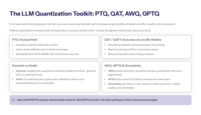
• Post-Training Quantization (PTQ): Quantize a trained model; fast to deploy.

• Quantization-Aware Training (QAT): Simulate quantization during training; best for maintaining accuracy.

• Dynamic Quantization: Quantize activations at runtime; convenient on CPUs.

• Static Quantization: Fix scales/zero-points ahead of time using calibration.

Each family contains many different quantization methods and heuristics; selecting among them depends on latency targets, hardware support, and tolerance for fine-tuning.

Post-Training Quantization (PTQ)

PTQ converts weights (and optionally activations) after training, using a small calibration dataset to estimate ranges. For LLMs, PTQ often uses:

• Per-channel weight quantization for linear layers (lower quantization error than per-tensor).

• KL-divergence or MSE-based range selection.

• Scale quantization strategies that minimize error in high-leverage channels.

PTQ is attractive because you don’t touch training data or retrain the machine learning model; you simply perform quantization on the checkpoint and measure quality.

Quantization-Aware Training (QAT)

QAT places “fake-quant” operators in the forward pass so the network learns under quantized conditions. During backprop, gradients flow through straight-through estimators, and final weights are saved in low precision.

Benefits:

• Best chance to recover accuracy at low bit-widths (e.g., 4-bit).

• Can co-learn scales/zero-points and optionally use activation-aware weight quantization schedules.

• Supports fine tuning for minimal accuracy loss.

Costs:

• Requires training data access and compute.

• Longer cycles than PTQ.

Dynamic vs. Static Quantization

Dynamic quantization converts weights offline (usually to INT8) while computing activation scales on the fly, adapting to input context statistics. It’s convenient for CPU inference with linear layers and delivers less computational costs without calibration.

Static quantization fixes both weight and activation parameters ahead of time—after a calibration pass—yielding more predictable latency and better throughput on accelerators.

Activation-Aware Weight Quantization (AWQ) & GPTQ

Two LLM-oriented PTQ approaches have proven effective:

• AWQ (Activation-Aware Weight Quantization): Selects and protects a small subset of critical channels based on activation sensitivity, then quantizes the rest more aggressively—reducing quantization error where it matters most.

• GPTQ (Groupwise/Blockwise PTQ): Uses second-order approximations to minimize output error when quantizing groups of weights. This is a form of block wise quantization tuned to transformer linear layers.

Both methods are designed for neural networks with attention/MLP blocks and often yield strong W4A16 or W4A8 results with modest quality drop.

Granularity: Layer-Wise, Block-Wise, Group-Wise

Quantization granularity is a powerful knob:

• Layer wise quantization: Single scale per tensor; simplest but highest error.

• Per-channel (or per-column/row): Separate scales per output/input channel; strong default for GEMMs.

• Block wise quantization: Partition weights into small blocks (e.g., 64 or 128) with individual scales; balances performance and accuracy.

Finer granularity often improves quality but adds metadata and compute overhead during de/quantize.

Affine Quantization in Practice: Scale & Zero-Point Tuning

In INT8 affine schemes, choose the scaling factor s to map min/max to integer maximum values while avoiding outlier clipping. For symmetric quantization, z=0; for asymmetric, z centers zero to improve bias handling. Practical tips:

• Use percentile clipping (e.g., 99.9th) to avoid outlier-driven scales.

• Prefer per-channel scales for weight tensors.

• Store scales in FP16/FP32; keep fast integer kernels for matmuls.

These details, while rooted in signal processing, are what keep quantized weights numerically stable.

Choosing Bit-Widths: W8A8, W4A8, and Beyond

• W8A8 (INT8 weights/activations): Widely supported, strong accuracy, easy win.

• W4A16 or W4A8: Larger savings; requires PTQ/QAT tricks (AWQ, GPTQ) to curb quantization error.

• Ternary/Binary: Research-grade extreme quantization; massive savings with steep quality risks for LLMs.

As bit-width falls, quantization difficulty rises. If you must push below 8-bit, expect to combine per-channel scaling, outlier handling, and fine tuning.

Quantization for Attention and KV Cache

Attention is sensitive to small perturbations. Practical recipes include:

• Keep model weights in low precision but retain softmax-critical paths (e.g., attention logits) at higher precision to avoid overflow.

• Quantize K/V caches with per-head or per-sequence scales to hold memory down while preserving retrieval quality.

• Use mixed precision for layer norms and residual adds to limit accumulation error.

These selective policies reduce quantization error where it most affects model accuracy.

Calibration Dataset & the Steps to Perform Quantization

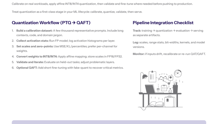
For PTQ/static schemes, build a calibration dataset of a few thousand representative prompts. Avoid only “easy” text—include long contexts, code blocks, and domain jargon.

Quantization procedure (PTQ static)

1. Collect calibration batches from real workloads.

2. Run the unquantized model to gather activation histograms.

3. Estimate ranges (MSE, KL, percentile) and set per-tensor/per-channel scales.

4. Convert weights to quantized weights (e.g., INT8).

5. Validate on a held-out set; iterate ranges for layers with larger quantization errors.

6. Optionally fine tune briefly (QAT-style) to recover tail metrics.

This is the practical “how” to perform quantization with minimal accuracy loss.

Fine Tuning After Quantization (QAFT)

When PTQ alone underperforms, add a brief fine tuning phase with fake-quant ops (sometimes called QAFT):

• Freeze most layers; adjust sensitive blocks.

• Train with a small LR on a task-specific or mixed dataset.

• Target layers that dominate error (often attention projections and MLPs).

This hybrid approach frequently restores metrics while keeping the smaller models and speed benefits you want.

Measuring Impact: Model Size, Latency, Energy

Quantization benefits are tangible:

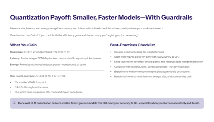
• Model size. INT8 cuts parameter storage by ~2× vs. FP16; INT4 cuts ~4×.

• Latency. Integer GEMMs + reduced memory traffic lower token inference time.

• Energy. Fewer bytes moved → less power, which compounds at scale.

Track gains alongside quality to ensure you’re maintaining accuracy where it matters (e.g., exactness for math/code, factuality for QA).

Symmetric vs. Asymmetric Quantization

• Symmetric quantization: [-S, S] mapped to signed integers; simple and fast; great when distributions are centered.

• Asymmetric quantization: adds zero point to better represent skewed ranges; helpful for activations with strong positive bias.

Experiment—many transformer layers prefer symmetric for weights and asymmetric for activations.

Hardware & Kernel Support

Performance depends on kernels:

• CPUs: dynamic quantization and INT8 GEMMs are mature; good for serverless endpoints.

• GPUs: Vendor libraries accelerate INT8/FP8 and support per-channel scales; INT4 support varies.

• NPUs/ASICs: Some expose native low-bit dot-product ops explicitly tuned for language models.

Choose a path aligned with your serving stack; the fastest scheme on paper may underperform without matching kernels.

Integration in a Machine Learning Pipeline

Treat quantization as a first-class stage in your machine learning lifecycle:

• Train (FP32/BF16) → Quantize (PTQ/QAT) → Evaluate → Serve.

• Log scales, range estimation stats, and versioned artifacts for reproducibility.

• Monitor drift; if inputs shift, recalibrate ranges or re-run QAT.

For many neural networks, quantization is routine hygiene akin to pruning or distillation.

Troubleshooting & Pitfalls

• Quality drops unexpectedly? Check that calibration covers long tails; adopt per-channel scaling.

• Unstable logits? Keep layernorm/residuals in higher precision.

• Outlier channels? Use AWQ/GPTQ to shield them.

• Attention collapse? Quantize K/V carefully; consider higher precision for softmax inputs.

• Blocked by kernels? Your gains depend on vendor quantization methods and optimized paths.

Document your quantization methods and retry with alternative common quantization techniques when necessary.

Case Snapshot: INT8 PTQ on a 7B LLM

• Baseline: BF16 weights/activations, ~14 GB VRAM.

• PTQ: W8A8 per-channel weights, asymmetric activations, 2k-sample calibration dataset.

• Results: ~2× smaller footprint; ~1.4–1.6× throughput lift; <0.5-point drop on general QA; modest drop on code unless adding small fine tuning.

  This illustrates the default trade-off curve many teams see when they perform quantization conservatively.

Research & Community (NeurIPS and Beyond)

Many innovations in LLM quantization appear at Neural Information Processing Systems (NeurIPS) and similar venues, covering FP8 training, outlier handling, activation-aware weight quantization, and block wise quantization for transformers. Keeping up with these proceedings helps you track state of the art and new common quantization techniques.

Checklist: Best Practices to Achieve Quantization with Minimal Accuracy Loss

• Use per-channel scaling for weight tensors.

• Prefer symmetric for weights; test asymmetric for activations.

• Calibrate with representative, long-context prompts.

• Keep layernorm/softmax in higher precision.

• Start with W8A8; push to W4 only with AWQ/GPTQ or QAT.

• Add short fine tuning if critical metrics regress.

• Benchmark end-to-end (latency, energy, model size, accuracy).

Frequently Asked Questions

This FAQ section addresses common questions about what is LLM quantization and how quantization occurs in large language models. We cover key concepts such as the transformation of high precision values—often represented as floating point numbers—into discrete values suitable for lower precision data types.

Understanding these processes, including the role of bit floating point formats and the importance of quantization parameters like scaling factor and zero point, is essential for grasping how quantization improves model efficiency while maintaining accuracy.

What is the affine quantization scheme, and why is it important?

The affine quantization scheme is a popular quantization technique that maps continuous real-valued parameters to quantized values using quantization parameters such as the scaling factor and zero point. This approach enables efficient representation of weights and activations in lower precision data types while minimizing quantization error, which is crucial for maintaining model accuracy in LLMs.

How does the weight conversion process affect model quantization?

The weight conversion process involves transforming high precision model weights into quantized weights by applying the scaling factor and zero point. This process directly impacts the quality of the quantized model, as improper conversion can introduce larger quantization errors, leading to degraded model accuracy. Careful calibration and selection of quantization parameters are essential to optimize this process.

What role does matrix multiplication play in LLM quantization?

Matrix multiplication is a fundamental operation in neural networks, including LLMs, where quantized weights and activations are multiplied during inference. Efficient quantization reduces the bit width of operands involved in matrix multiplication, lowering computational demands and memory bandwidth usage, which accelerates inference and reduces energy consumption on hardware.

How does the quantization process handle input data during inference?

During inference, the quantization process converts input data activations from high precision to quantized values using predetermined quantization parameters. This ensures that the model operates entirely within lower precision formats, enabling faster and more efficient computation. Dynamic quantization techniques may adjust these parameters on the fly based on input data distribution to optimize accuracy.

Is PTQ enough for most LLMs?

Often yes for INT8 (W8A8). For INT4 or strict domains (code/math), add AWQ/GPTQ or brief QAT.

What’s the role of a calibration dataset?

It drives stable range estimation for activations. Poor calibration ⇒ larger quantization errors.

Symmetric or asymmetric—how do I choose?

Try symmetric for weights, asymmetric for activations; verify on your workload.

Can I quantize everything to 4-bit?

That’s extreme quantization. It can work with the right recipe but carries higher quantization difficulty.

Will quantization help on GPU?

Yes—INT8 kernels and reduced memory bandwidth improve throughput, especially for batch inference.

Do I need to change my training?

Not with PTQ. With QAT/QAFT, you’ll retrain briefly to learn under quantized noise.

Conclusion

LLM quantization compresses models into lower precision formats to unlock faster, cheaper, greener inference—without sacrificing too much model accuracy. By combining robust affine quantization (well-chosen scaling factor and zero point), careful range estimation, and LLM-specific techniques like AWQ/GPTQ, teams can deliver smaller models that meet production SLOs.

Start with conservative INT8 weight quantization and activation quantization, validate on a representative calibration dataset, and iterate. When quality matters most, bring in quantization-aware training or short fine tuning cycles to stabilize metrics. With the right quantization methods, you can maintain accuracy while cutting latency, memory, and energy—making state-of-the-art language models practical across platforms and scales.